What you will learn
Read a tiny image as numbers and calculate the response of a local contrast filter.
Before you begin: basic arithmetic, scientific notation and curiosity.

Begin with the mug
In the opening picture, the mug feels like one object. In an image file it is spread across many samples. Each pixel records numerical values, often red, green and blue channels. Those values are influenced by illumination, material, camera settings and processing. The machine does not receive the word “mug” along with those pixels. A learning system has to connect patterns in the numbers with the task we ask it to perform.
Look at a small neighbourhood
Before thinking about a large neural network, take three neighbouring brightness values. A simple filter can compare the left and right values. If they differ sharply, you may be near an edge. Slide the same filter across a row and you obtain a sequence of responses. This is the basic intuition behind a local operation: each output looks at a small region, rather than trying to interpret the entire scene at once.
Edges are clues, not objects
An edge response could come from the mug boundary, a shadow, the notebook or an exposure change. It does not tell you which one. That is why a single filter is useful but insufficient. In a learned vision system, later operations combine local responses into representations that can support a task. Even then, a feature that helps on training images may fail when the background or lighting changes. A sharp response is evidence of contrast, not understanding.
Do one calculation slowly
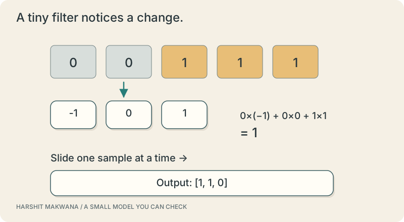
Use the row [0, 0, 1, 1, 1] and the three-value filter [−1, 0, 1]. Multiply matching entries and add, then shift one place. We will use cross-correlation, which does not reverse the filter; many deep-learning libraries call this operation convolution. Keeping that convention explicit prevents a sign surprise. Once this tiny example feels ordinary, a grid of filters and multiple image channels is a manageable extension rather than a leap of faith.
SEE THE RELATIONSHIPS
From structure to behavior.
MAKE THE IDEA PRECISE
The mathematics.
| Symbol | Meaning |
|---|---|
| left, centre, right | Three adjacent brightness values, normalised here to 0…1 |
| response | Signed local contrast response |
Build the equation, step by step
- Align the filter with three consecutive samples. Multiply each sample by its corresponding weight.
- Add the products to obtain one output. For [0,0,1], the result is 1.
- Move the window by one sample. With length 5, filter width 3, stride 1 and no padding, there are 3 valid outputs.
WORK THROUGH THE NUMBERS
Worked example
The three windows produce [1, 1, 0]. The first two see a change from dark to bright; the last window is constant and gives zero. Reversing the filter reverses the sign of the edge response.
A small Python experiment.
Python 3 · Standard library only · Synthetic educational example. Run this in your own notebook or a local file.
row = [0, 0, 1, 1, 1]
kernel = [-1, 0, 1]
result = [sum(row[i+j]*kernel[j] for j in range(3)) for i in range(3)]
print(result)
Expected output
[1, 1, 0]
Change one quantity, predict the result, and then run the code again. Explain any difference before adding complexity.
Test your understanding.
Try it: Add 0.2 to every brightness value without clipping. Predict whether the filter response changes, then check it.
Self-check: Why does a constant brightness offset cancel in this example?
The filter weights add to zero. Adding the same offset to all three samples adds the offset multiplied by that zero sum, leaving the response unchanged. This property belongs to this linear filter; it does not make an entire vision system immune to illumination changes.
Where this model stops: This one-dimensional synthetic row leaves out colour, noise, camera geometry and boundaries of a two-dimensional image.
A research question: Keep one assumption fixed and change another. What observation would make you revise your explanation?
Record evidence in your mastery worksheet →Read with the original sources.
These readings support the concepts and deeper investigation. The worked numbers and illustrations above are teaching examples.
Primary source / official teaching material
Stanford CS231n — Convolutional neural networks ↗
Reference for local receptive fields, shared filters and convolutional network structure.