What you will learn
Connect a circuit expectation to a loss, then check a parameter-shift gradient.
Before you begin: Putting data into a circuit
A circuit with something to adjust
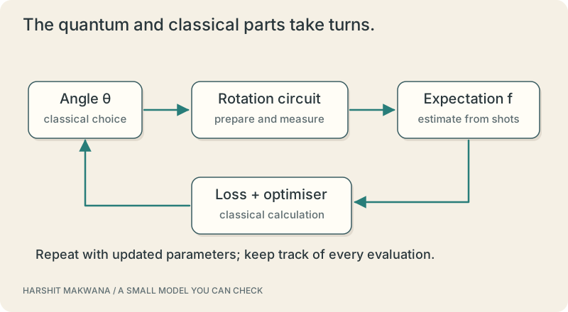
Imagine a circuit with a rotation angle θ that you are allowed to change. Run the circuit, measure an observable, and obtain an estimated output. If that output is not what you want, adjust θ and try again. This is the basic rhythm of a variational model. The word sounds elaborate, but the training loop is familiar: make a prediction, measure a loss, use information about the loss to change the parameters.
Keep one clean example
Prepare |0⟩, rotate around Y by θ, and measure Z, whose outcomes are +1 and −1. The ideal expected value is cos θ. Suppose our target expectation is zero. A squared-error loss is then cos²θ, which reaches zero at π/2. We can inspect every part of this tiny problem. It is a useful place to learn the difference between a circuit parameter, an expectation value and the loss that a classical optimiser receives.
A gradient from shifted circuits
For this rotation and observable, the derivative of the expectation can be obtained from two shifted parameter values, θ+π/2 and θ−π/2. Their difference, divided by two, equals −sin θ. That is a parameter-shift rule. The rule has conditions; it is not a licence to shift every arbitrary function by the same amount. To differentiate the squared loss, we still need the chain rule around the expectation.
Where the tidy picture gets rough
The script below uses exact cosines. Hardware would estimate the expectation from a finite number of shots, so both the output and the estimated gradient fluctuate. Extra circuit parameters bring more evaluations, and a difficult loss landscape can make training frustrating. Before increasing the circuit size, ask whether your small implementation matches a calculation you can do on paper. A trustworthy tiny model is a better starting point than a mysterious large one.
SEE THE RELATIONSHIPS
From structure to behavior.
MAKE THE IDEA PRECISE
The mathematics.
| Symbol | Meaning |
|---|---|
| θ | Trainable Y-rotation angle, radians |
| f | Expected Z measurement, between −1 and +1 |
| f′ | Derivative with respect to the angle |
Build the equation, step by step
- A Y rotation prepares probabilities cos²(θ/2) and sin²(θ/2). Weight them by the Z outcomes +1 and −1.
- Their difference is cos θ. Evaluating the two shifted cosines gives −sin θ after subtraction and division by two.
- For L=(f−y)², apply the chain rule: dL/dθ=2(f−y)f′. The gradient of the expectation is not automatically the gradient of the loss.
WORK THROUGH THE NUMBERS
Worked example
At θ=π/3, f=0.5 and f′≈−0.866. With target y=0, the loss is 0.25 and its derivative is approximately −0.866. A sufficiently small step in the positive θ direction decreases this local loss.
A small Python experiment.
Python 3 · Standard library only · Synthetic educational example. Run this in your own notebook or a local file.
from math import cos, pi
theta = pi/3
f = cos(theta)
grad = (cos(theta+pi/2)-cos(theta-pi/2))/2
print(f"expectation = {f:.3f}")
print(f"loss = {f*f:.3f}; loss gradient = {2*f*grad:.3f}")
Expected output
expectation = 0.500
loss = 0.250; loss gradient = -0.866
Change one quantity, predict the result, and then run the code again. Explain any difference before adding complexity.
Test your understanding.
Try it: Try θ=0 and θ=π/2. Which has a zero gradient, and does that alone tell you whether the loss is small?
Self-check: Does a zero gradient mean the model has found a useful solution?
No. In this example both θ=0 and θ=π/2 have zero loss gradient, but their losses are 1 and 0. A stationary point can be a maximum, minimum or another difficult region. Inspect the objective and nearby behaviour instead of treating zero gradient as a certificate of success.
Where this model stops: Only a single ideal rotation is simulated. Finite-shot gradients, noisy gates and multi-parameter optimisation require additional analysis.
A research question: Keep one assumption fixed and change another. What observation would make you revise your explanation?
Record evidence in your mastery worksheet →Read with the original sources.
These readings support the concepts and deeper investigation. The worked numbers and illustrations above are teaching examples.
Primary source / official teaching material
Schuld et al. — Evaluating analytic gradients on quantum hardware ↗
Primary derivation of parameter-shift methods and their conditions; our example is a single analytic rotation.
Primary source / official teaching material
IBM Quantum Learning — Single systems ↗
Background for states, amplitudes, measurements and the Hadamard operation.