What you will learn
Explain units, solve an RC response, implement an Euler step, and defend a simple statistical comparison.
Before you begin: basic arithmetic, scientific notation and curiosity.
Begin with a quantity you can measure
A voltage is a difference in electrical potential, not a material flowing through a wire. Current measures charge crossing a boundary per unit time. An ion is an atom or molecule with a net charge; Na+ and K+ carry one positive elementary charge, Ca2+ carries two, and Cl- carries one negative charge. Write the measurement and its unit together. A number such as 20 is not a membrane timescale until you say whether it means seconds or milliseconds.
A useful circuit picture
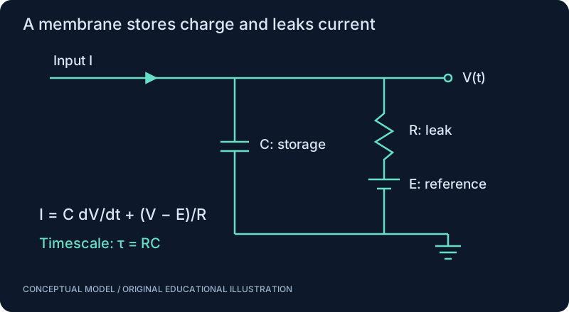
Imagine a container that can store water while a small opening lets water escape. Storage and leakage compete. A membrane can be approximated as electrical storage plus a leakage pathway, although the water analogy does not explain selective ion channels. Capacitance relates stored charge to voltage; resistance relates voltage difference to current. Their product has units of time. The illustration below separates the circuit quantities so that the algebra has a physical meaning.
From biology to a neural computation
A passive membrane has memory: its voltage depends on recent input rather than only the current sample. A neural network with state can similarly integrate weak evidence across time. Before discussing intelligence, ask whether the model preserves the relevant timescale. A simulator stepping once per second cannot resolve a 20-millisecond process reliably. Numerical convergence is part of the model, not cosmetic cleanup.
Your first derivation
Current conservation gives I = I_leak + I_capacitor. With a leak reference E, I_leak = (V - E)/R and I_capacitor = C dV/dt. Substitute these expressions and multiply by R to obtain the membrane equation used later. This derivation assumes a constant resistance and capacitance; biological conductances can vary with voltage, time and chemical state.
SEE THE RELATIONSHIPS
From structure to behavior.
MAKE THE IDEA PRECISE
The mathematics.
| Symbol | Meaning |
|---|---|
| tau | Time constant, seconds |
| R | Resistance, ohms |
| C | Capacitance, farads |
| V | Voltage difference, volts |
| I | Current, amperes |
| Q | Charge, coulombs |
Build the equation, step by step
- Start with Q = CV: at fixed capacitance, doubling the voltage difference doubles the stored charge. Differentiate with respect to time to obtain the capacitive current C dV/dt.
- For the parallel leak pathway, the voltage across the resistor is V − E, so its current is (V − E)/R. Add the two currents and equate their sum to the injected current.
- Multiplying by R gives RC dV/dt = −(V − E) + RI. Define τ = RC. With no input, displacement from E decays exponentially; after one τ, about 36.8% remains.
WORK THROUGH THE NUMBERS
Worked example
Choose an illustrative resistance of 100 megaohms and capacitance of 200 picofarads. Their product is 0.020 seconds = 20 milliseconds. A 0.1-nanoamp current through that resistance gives a 10-millivolt drop. These are chosen example values, not measurements of a particular fly neuron.
A small Python experiment.
Python 3 · Standard library only · Synthetic educational example. Run this in your own notebook or a local file.
R = 100e6       # ohms
C = 200e-12     # farads
I = 0.1e-9      # amperes
print(f"tau = {R*C*1000:.1f} ms")
print(f"I R = {I*R*1000:.1f} mV")
Expected output
tau = 20.0 ms
I R = 10.0 mV
Change one quantity, predict the result, and then run the code again. Explain any difference before adding complexity.
Test your understanding.
Try it: Double C while keeping R and I fixed. Predict which output changes before running the example. Explain why the steady resistor drop does not change.
Self-check: Does doubling R always double the final voltage?
Only the voltage displacement produced by a fixed injected current doubles in this passive model. The reference E remains. If C is fixed, the time constant also doubles, so the approach to equilibrium becomes slower. Real channels may invalidate the constant-resistance assumption.
Where this model stops: A passive circuit cannot generate a biological action potential. A fixed time constant is a modeling choice, not a universal neuron property.
A research question: Which measurements would reveal that a constant-conductance model is inadequate?
Record evidence in your mastery worksheet →THE NEXT LAYER
Chapter depth map.
This introduction provides a first model. The following chapters are outlines for deeper future editions; their full treatments have not yet been published.
Physical intuition
1.1 Atoms, ions and electrical quantities · Outline
- 1.1.1 Atoms and valence: Na+, K+, Ca2+ and Cl-
- 1.1.2 Charge and the coulomb
- 1.1.3 Voltage as energy per charge; reference potentials
- 1.1.4 Current as charge flow; conventional current and ion movement
- 1.1.5 Resistance, conductance and dimensional analysis
1.2 Capacitance and the RC circuit · Outline
- 1.2.1 Charge storage and C = Q/V
- 1.2.2 Resistor and capacitor circuit diagrams
- 1.2.3 Kirchhoff current balance
- 1.2.4 Time constant tau = RC and step responses
- 1.2.5 Worked unit conversions: megohms, picofarads, nanoamps and milliseconds
The mathematics of change
1.3 Calculus and differential equations · Outline
- 1.3.1 Functions, graphs, slopes and derivatives
- 1.3.2 Integrals as accumulation
- 1.3.3 First-order differential equations and initial conditions
- 1.3.4 Exponential relaxation and analytic solutions
- 1.3.5 Euler integration, truncation error and timestep convergence
1.4 Vectors, matrices and graphs · Outline
- 1.4.1 Vectors, dot products and norms
- 1.4.2 Matrix multiplication and coordinate transformations
- 1.4.3 Eigenvalues, modes and local stability
- 1.4.4 Directed weighted graphs and adjacency conventions
- 1.4.5 Sparse matrices and algorithmic cost
Uncertainty and scientific computation
1.5 Probability and statistics · Outline
- 1.5.1 Random variables and conditional probability
- 1.5.2 Bayes rule and likelihood
- 1.5.3 Bernoulli, Poisson and Gaussian models
- 1.5.4 Estimation, confidence intervals and effect sizes
- 1.5.5 Independent samples, controls, seeds and reproducible Python
1.6 Dynamical systems and information · Outline
- 1.6.1 State spaces, equilibria and phase portraits
- 1.6.2 Feedback, oscillations and stability
- 1.6.3 Entropy and mutual information with assumptions
- 1.6.4 Sampling, aliasing and temporal resolution
- 1.6.5 Optimization, gradients and constrained model fitting
Read with the original sources.
These readings support the concepts and deeper investigation. The worked numbers and illustrations above are teaching examples.
Author-hosted textbook
Neuronal Dynamics — Gerstner, Kistler, Naud & Paninski (2014) ↗
Use for neuron-model prerequisites and notation; this site provides an original curriculum, not a reproduction of the textbook.
Author-hosted textbook
Gerstner et al. — passive membrane and integrate-and-fire equations ↗
Reference for the passive-membrane approximation and integrate-and-fire conventions.