What you will learn
Draw a neuron, explain membrane currents, and distinguish synaptic mechanisms from abstract weights.
Before you begin: Foundations: matter, mathematics & computation
Read the cell as interacting compartments
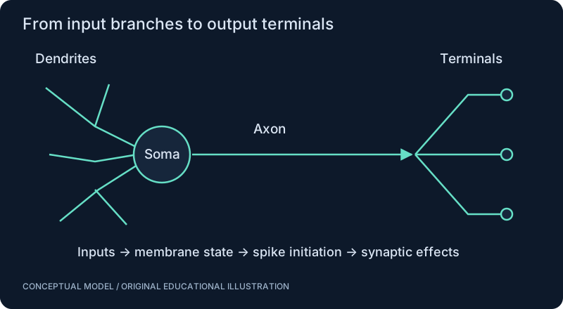
Dendrites, the cell body and the axon describe structure, but a diagram alone does not specify how every neuron behaves. The familiar branched cartoon is a teaching abstraction; many fly neurons have different geometries. Membrane potential is measured across a membrane. When channels open, ion movement depends on both concentration and electrical differences. Depolarization means the potential becomes less negative relative to the chosen reference.
A spike is an event with a mechanism
Action potentials involve changing conductances and regenerative feedback. A computational spike timestamp keeps the event while discarding its waveform. That reduction can be useful when timing is the question, and inappropriate when channel dynamics are the question. Refractoriness limits responsiveness after activity; it should be specified explicitly rather than inferred from a plotting convention.
From synapse to network weight
A chemical synapse is not simply a signed number. Transmitter release, receptors, reversal potentials, timing and postsynaptic state shape its effect. A scalar artificial weight compresses these mechanisms into a task-dependent approximation. Excitation and inhibition should therefore be explained through effect and context. A predicted transmitter label in a connectome does not, by itself, measure every downstream response.
Reading a population
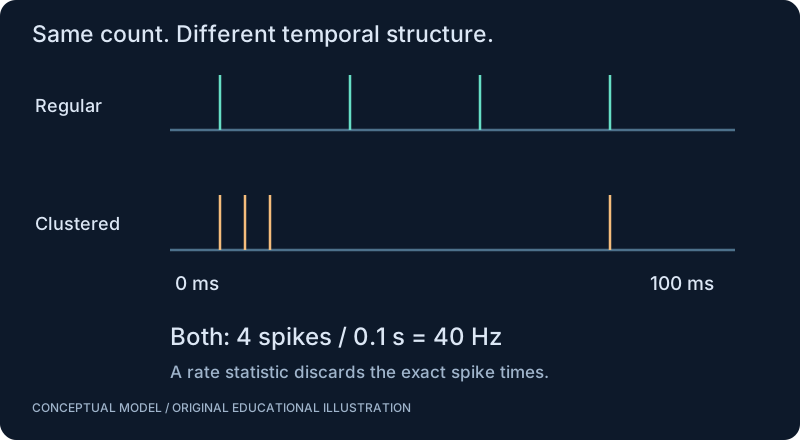
Rate and timing are different descriptions of the same spike train. A count over 100 milliseconds loses the order of the events. A population decoder may recover information that any one cell does not provide. To choose a representation, define the behavior and the observation window first, then test whether information survives your simplification.
SEE THE RELATIONSHIPS
From structure to behavior.
MAKE THE IDEA PRECISE
The mathematics.
| Symbol | Meaning |
|---|---|
| r | Average firing rate, spikes per second (Hz) |
| N | Number of observed spikes |
| T | Observation duration, seconds |
Build the equation, step by step
- Choose the observation window before counting. A count without a duration cannot define a rate.
- Divide the spike count N by window length T in seconds. The resulting unit is spikes per second, conventionally reported in hertz.
- Changing the window changes the estimate. A longer window reduces time resolution; a short window can be dominated by whether a single spike fell just inside or outside its boundary.
WORK THROUGH THE NUMBERS
Worked example
Five spikes in 0.1 seconds give 50 Hz. This does not mean spikes are exactly 20 ms apart. Two trains can have identical counts and very different event timing.
A small Python experiment.
Python 3 · Standard library only · Synthetic educational example. Run this in your own notebook or a local file.
spikes_ms = [4, 6, 20, 70, 98]
window_ms = 100
rate_hz = len(spikes_ms) / (window_ms / 1000)
intervals = [b-a for a,b in zip(spikes_ms, spikes_ms[1:])]
print(f"rate = {rate_hz:.0f} Hz; intervals = {intervals} ms")
Expected output
rate = 50 Hz; intervals = [2, 14, 50, 28] ms
Change one quantity, predict the result, and then run the code again. Explain any difference before adding complexity.
Test your understanding.
Try it: Create a second five-spike train with evenly spaced events. Compare rates and inter-spike intervals.
Self-check: Can equal firing rates imply different messages?
Yes. Equal counts in equal windows give equal average rates but may have different spike timing, intervals or correlations with other cells. Whether those differences carry useful information depends on the downstream mechanism and task; timing is not automatically meaningful.
Where this model stops: A firing rate is a summary, not a complete neural code. Do not identify artificial activation values with measured biological signals without defining the mapping.
A research question: For a rapid reflex, when does a spike-count window become too slow?
Record evidence in your mastery worksheet →THE NEXT LAYER
Chapter depth map.
This introduction provides a first model. The following chapters are outlines for deeper future editions; their full treatments have not yet been published.
Cells and signals
2.1 A cell built for communication · Outline
- 2.1.1 Cells, membranes and intracellular compartments
- 2.1.2 Dendrites, soma, axon and axon hillock
- 2.1.3 Ion concentrations and selective channels
- 2.1.4 Resting potential and electrochemical gradients
- 2.1.5 Glia and the limits of a neuron-only account
2.2 From voltage to action potential · Outline
- 2.2.1 Depolarization, repolarization and hyperpolarization
- 2.2.2 Sodium and potassium conductance changes
- 2.2.3 Action potential initiation and propagation
- 2.2.4 Absolute and relative refractory periods
- 2.2.5 Graded potentials and species-specific physiology
Communication and adaptation
2.3 Synapses and plasticity · Outline
- 2.3.1 Chemical and electrical synapses
- 2.3.2 Calcium, transmitter release and receptors
- 2.3.3 Excitatory and inhibitory effects depend on reversal potentials
- 2.3.4 Neuromodulation, Hebbian learning and STDP
- 2.3.5 Homeostasis and plasticity across timescales
2.4 Neural codes and measurements · Outline
- 2.4.1 Spike frequency and rate coding
- 2.4.2 Spike timing and temporal coding
- 2.4.3 Population codes and decoding
- 2.4.4 Synchronization and correlated activity
- 2.4.5 Recording methods, measurement noise and interpretation
Read with the original sources.
These readings support the concepts and deeper investigation. The worked numbers and illustrations above are teaching examples.
Primary paper
Hodgkin & Huxley (1952): membrane-current model ↗
A mechanistic modeling milestone. Read after RC circuits and differential equations; distinguish squid-axon measurements from universal neuron parameters.
Author-hosted textbook
Neuronal Dynamics — Gerstner, Kistler, Naud & Paninski (2014) ↗
Use for neuron-model prerequisites and notation; this site provides an original curriculum, not a reproduction of the textbook.