What you will learn
Compare feedforward and recurrent circuits using explicit inputs, states, outputs, and perturbations.
Before you begin: Biological neuroscience
The interaction is the computation
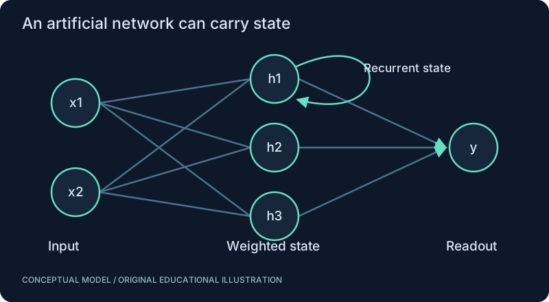
A circuit combines inputs, internal state and outputs. In a feedforward network, activity moves through successive transformations. Recurrent connections allow past activity to influence the next state. A reflex is better understood as a loop through sensing, circuitry, body and environment than as a chain that ends at a motor command.
Inhibition can improve a representation
Suppose neighboring units respond to similar inputs. Subtracting a fraction of neighboring activity can emphasize differences. This is a toy contrast computation, not a claim that every biological inhibitory circuit implements the same rule. A small circuit can reveal a useful computational motif while leaving its detailed physiology unresolved.
Feedback can stabilize or amplify
In a linear recurrent toy, each step multiplies previous activity by a gain. Gains smaller than one in magnitude make the zero-input state decay; gains greater than one can amplify it without bound. Real networks introduce nonlinearities, multiple modes, noise and regulation. The simple calculation teaches why connectivity and dynamics must be studied together.
A neural-network perspective
Recurrence supplies a form of state without requiring a database. It can support integration and temporary retention, but does not automatically produce memory with useful capacity or robust decisions. Test the circuit with pulses, distractors and missing input. For robotics, include the actuator and sensor delays in the feedback loop.
SEE THE RELATIONSHIPS
From structure to behavior.
MAKE THE IDEA PRECISE
The mathematics.
| Symbol | Meaning |
|---|---|
| x_t | Scalar circuit state at time step t |
| a | Recurrent retention gain, dimensionless |
| b | Input gain |
| u_t | External input at time step t |
Build the equation, step by step
- Separate the previous state contribution a x from the input contribution b u. This is a discrete linear approximation, not an anatomical identity.
- Set u to zero and apply the rule repeatedly: x after k steps equals a to the power k times the initial state.
- For this scalar model, magnitudes shrink when |a| < 1. A negative a alternates the sign. At |a| > 1, magnitudes grow unless a nonlinear limit intervenes.
WORK THROUGH THE NUMBERS
Worked example
With no new input and a = 0.8, an initial state of 1 becomes 0.8, 0.64 and 0.512. These are exact updates of this discrete model, not a fitted biological decay.
A small Python experiment.
Python 3 · Standard library only · Synthetic educational example. Run this in your own notebook or a local file.
x = 1.0
values = []
for _ in range(3):
    x = 0.8*x
    values.append(round(x, 3))
print(values)
Expected output
[0.8, 0.64, 0.512]
Change one quantity, predict the result, and then run the code again. Explain any difference before adding complexity.
Test your understanding.
Try it: Try a = -0.8 and a = 1.1. Explain alternating decay versus growth.
Self-check: Why does a stable recurrent circuit still need input?
Stability means disturbances do not grow without bound; it does not mean useful activity appears spontaneously. With |a| < 1 and no new input, this model forgets its initial state. Persistent memory needs an appropriate mechanism, not just the word recurrence.
Where this model stops: One scalar stability condition does not establish stability of a large nonlinear circuit.
A research question: Can a recurrent motif retain useful information while rejecting irrelevant perturbations?
Record evidence in your mastery worksheet →THE NEXT LAYER
Chapter depth map.
This introduction provides a first model. The following chapters are outlines for deeper future editions; their full treatments have not yet been published.
Circuit building blocks
3.1 Small circuits, useful computations · Outline
- 3.1.1 Neural circuits and microcircuits
- 3.1.2 Feedforward chains and convergence
- 3.1.3 Recurrent excitation and inhibition
- 3.1.4 Lateral inhibition and competition
- 3.1.5 Input-output curves and causal perturbations
3.2 Sensing and moving · Outline
- 3.2.1 Sensory transduction and sensory pathways
- 3.2.2 Motor neurons and motor systems
- 3.2.3 Reflex arcs and feedback loops
- 3.2.4 Central pattern generators and rhythmic behavior
- 3.2.5 Body and environment as part of the closed loop
Coordination over time
3.3 Choosing, attending and navigating · Outline
- 3.3.1 Decision circuits and evidence accumulation
- 3.3.2 Attention-like selection without anthropomorphism
- 3.3.3 Heading and navigation representations
- 3.3.4 Feedforward predictions versus feedback corrections
- 3.3.5 Distinguishing behavioral evidence from circuit speculation
3.4 Remembering and stabilizing · Outline
- 3.4.1 Persistent activity and memory circuits
- 3.4.2 Attractor dynamics and noise
- 3.4.3 Gain control and homeostatic regulation
- 3.4.4 Circuit lesions and model ablations
- 3.4.5 Emergence as a testable system property
Read with the original sources.
These readings support the concepts and deeper investigation. The worked numbers and illustrations above are teaching examples.
Author-hosted textbook
Neuronal Dynamics — Gerstner, Kistler, Naud & Paninski (2014) ↗
Use for neuron-model prerequisites and notation; this site provides an original curriculum, not a reproduction of the textbook.