What you will learn
Construct a directed graph and report which biological assumptions its weights do not encode.
Before you begin: Foundations: matter, mathematics & computation; Biological neuroscience
A map of connections
A connectome represents reconstructed neural connectivity. Let each neuron be a node and each directed synaptic connection an edge. Several synapses between a pair may be stored separately or aggregated into a weight. Choose and document that convention before computing statistics. An adjacency matrix is a coordinate system for a graph, so a row/column mistake can reverse every pathway in an otherwise correct program.
From images to a graph
Electron microscopy supplies images from which processes are segmented, traced, proofread and annotated. Each stage introduces uncertainty. Split errors can divide one cell; merge errors can join unrelated processes. A boundary can truncate connections. Treat release versions and reconstruction scope as part of the data, not a footnote added after the analysis.
Structure is a constraint, not a complete simulator
Synapse counts do not supply membrane constants, receptor effects, conduction delays, current activity or learning history. Building a neural model from a graph therefore requires extra assumptions. A good experiment changes those assumptions systematically and asks which conclusions survive. The architecture can be biologically grounded while the dynamics remain an engineered approximation.
Neural-network perspective
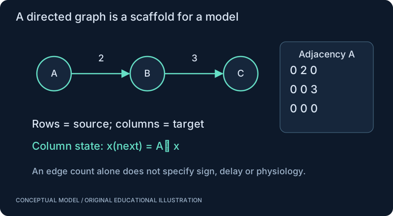
Here use A[i][j] for the connection from source i to target j. The input to target j is the sum over sources. Dense arrays store all pairs, including absent edges; sparse edge lists store the connections you actually use. On a large graph, format and orientation can determine whether a simulation is feasible.
SEE THE RELATIONSHIPS
From structure to behavior.
CHANGE A PARAMETER. TEST YOUR INTUITION.
Follow a signal through a directed graph
A synthetic chain A → B → C. Rows are sources and columns are targets. Change the A → B weight, then follow two synchronous propagation steps. No recurrence, leak or spikes are included.
Interactive controls load with JavaScript. The worked example below is available without it.
MAKE THE IDEA PRECISE
The mathematics.
| Symbol | Meaning |
|---|---|
| G | Directed graph |
| V | Set of neuron nodes; not membrane voltage in this equation |
| E | Set of directed edges |
| A_ij | Weight from source i to target j |
| x_i | Source activity |
| y_j | Accumulated target input |
Build the equation, step by step
- For every target j, collect contributions from all source nodes i. Multiply each source activity by its outgoing weight to that target.
- Sum those contributions to obtain y_j. With sources stored in rows, a column-vector implementation uses the transpose of A.
- Apply the operation twice to represent two propagation steps. This computes weighted paths of length two; it is not the same as moving signals through all edges instantaneously.
WORK THROUGH THE NUMBERS
Worked example
A synthetic chain has weight 2 from node 0 to 1 and weight 3 from node 1 to 2. Starting with activity only at node 0, one propagation step reaches node 1 and the next reaches node 2. This example intentionally has no decay or spike threshold.
A small Python experiment.
Python 3 · Standard library only · Synthetic educational example. Run this in your own notebook or a local file.
edges = [(0, 1, 2), (1, 2, 3)]
x = [1, 0, 0]
for _ in range(2):
    y = [0, 0, 0]
    for source, target, weight in edges:
        y[target] += weight*x[source]
    x = y
    print(x)
Expected output
[0, 2, 0]
[0, 0, 6]
Change one quantity, predict the result, and then run the code again. Explain any difference before adding complexity.
Test your understanding.
Try it: Reverse the two edges. Predict whether node 0 can still reach node 2.
Self-check: Does a large synapse count prove an excitatory connection?
No. Anatomy describes connectivity; sign and effect require transmitter, receptor, physiology and state information. The synthetic positive weights here illustrate graph arithmetic. They should not be substituted for inferred biological conductances.
Where this model stops: A strong or central anatomical connection is not proof of causal importance in every behavior.
A research question: How sensitive is your conclusion to uncertain edges or a different aggregation threshold?
Record evidence in your mastery worksheet →THE NEXT LAYER
Chapter depth map.
This introduction provides a first model. The following chapters are outlines for deeper future editions; their full treatments have not yet been published.
Representing structure
4.1 Neurons as a graph · Outline
- 4.1.1 G = (V, E): vertices, edges and metadata
- 4.1.2 Directed graphs, multigraphs and weighted graphs
- 4.1.3 Adjacency matrices with explicit row/column direction
- 4.1.4 Synapse counts versus physiological efficacy
- 4.1.5 Cell types, morphology, skeletons and brain regions
4.2 From microscopy to reconstruction · Outline
- 4.2.1 Electron microscopy and serial images
- 4.2.2 Segmentation and neuron tracing
- 4.2.3 Synapse detection and proofreading
- 4.2.4 Cell-type annotation and predicted neurotransmitters
- 4.2.5 Split/merge errors, missing boundaries and uncertainty
Asking graph questions
4.3 Paths, motifs and communities · Outline
- 4.3.1 Traversal and constrained pathway queries
- 4.3.2 In-degree, out-degree and centrality
- 4.3.3 Recurrent motifs and appropriate null models
- 4.3.4 Community detection and resolution dependence
- 4.3.5 Region aggregation and annotation bias
4.4 From structure to hypotheses · Outline
- 4.4.1 Connectivity does not specify dynamics
- 4.4.2 Delays, conductances and neuromodulators missing from a graph
- 4.4.3 Individual variation and incomplete reconstructions
- 4.4.4 Sensitivity analysis over uncertain edges
- 4.4.5 Tests relating topology to measured behavior
Read with the original sources.
These readings support the concepts and deeper investigation. The worked numbers and illustrations above are teaching examples.
Official dataset resource
FlyWire — official project and dataset resources ↗
An adult female fly brain resource. Record the exact release and annotation version; a brain dataset should not be described as a complete brain-and-body model.
Primary paper
Lin et al. (2024): network statistics of the fly connectome ↗
Study motif and network analysis with attention to filtering and null-model choices. Graph centrality is not automatically causal importance.
Official dataset resource
MaleCNS — official release and downloads ↗
The official download page exposes versioned data, including v1.0 resources. Keep specimen, release, filtering and annotation provenance with every derived graph.