Engineering project studio

What you will learn

Follow the project ladder alongside prerequisite parts; each project needs evidence, not a completion click.

Before you begin: Foundations: matter, mathematics & computation

Build a sequence of evidence

The project ladder progresses from one neuron to sparse networks, vision, connectome data and embodied simulation. Each step should produce a small artifact you can inspect: a voltage trace, a graph conversion, a confusion table or a controller log. More neurons are not a substitute for better tests.

Specify before scaling

Write the goal, model assumptions, units, dataset provenance, expected observations and a baseline. Keep experiment code, tests, configuration and results distinct. Use a manifest to identify data and versions. A benchmark without the parameters and inputs needed to rerun it is not yet a reproducible experiment.

Neural-network perspective

Connectivity storage is one scaling cost among several. Membrane state, delay queues, gradients and framework overhead can exceed the edge-array estimate. Measure a small model and extrapolate cautiously. Faster C++, CUDA, Rust or hardware implementations should be checked against a simple numerical reference before their outputs are trusted.

SEE THE RELATIONSHIPS

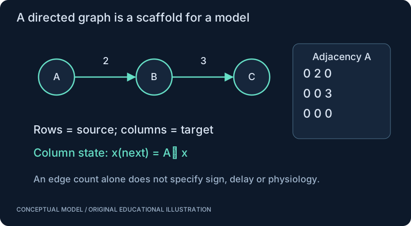
From structure to behavior.

Connectome: a labelled conceptual diagram — Figure 24.1 · Connectome. Original educational diagram; synthetic, not a measured result.

A learning flow for this part. Follow the assumptions through to an observable result.

MAKE THE IDEA PRECISE

The mathematics.

M = N d; sparse_bytes = M b_edge; dense_bytes = N² b_weight

Symbols and units
Symbol	Meaning
N	Number of neurons
d	Chosen average outgoing degree
M	Number of directed edges
b_edge	Illustrative bytes per stored edge
b_weight	Bytes per dense weight

Build the equation, step by step

For N nodes with average outgoing degree d, the number of directed edge records is N d when d is calculated over the same graph.
Multiply M by bytes per edge record for a sparse payload estimate. Multiply N squared by bytes per weight for the dense payload estimate.
These estimates omit allocator, index, metadata and runtime-state overhead unless included explicitly. Sparse storage reduces payload when M is small, but runtime speed also depends on access patterns and hardware.

WORK THROUGH THE NUMBERS

Worked example

For 1000 neurons with average degree 10, there are 10,000 edges. At an illustrative 8 bytes per edge, the edge payload is about 78.1 KiB. A float32 dense matrix uses about 3.8 MiB. Neither number includes all runtime overhead.

A small Python experiment.

Python 3 · Standard library only · Synthetic educational example. Run this in your own notebook or a local file.

N, degree = 1000, 10
sparse = N*degree*8
dense = N*N*4
print(f"edge payload = {sparse/1024:.1f} KiB; dense = {dense/1024**2:.1f} MiB")

Expected output

edge payload = 78.1 KiB; dense = 3.8 MiB

Change one quantity, predict the result, and then run the code again. Explain any difference before adding complexity.

Test your understanding.

Try it: Include one float32 membrane value per neuron and estimate the extra storage. What other arrays would a trained SNN require?

Self-check: Does a smaller sparse representation always execute faster?

No. Irregular indexing and scattered memory access can outweigh fewer arithmetic operations, while dense kernels can exploit specialized hardware. Measure representative workloads and include conversion costs; a storage estimate is not a speed benchmark.

Where this model stops: The example estimates storage, not throughput or end-to-end simulator memory.

A research question: Which optimization changes runtime while preserving the numerical behavior you care about?

Record evidence in your mastery worksheet →

THE NEXT LAYER

Chapter depth map.

This introduction provides a first model. The following chapters are outlines for deeper future editions; their full treatments have not yet been published.

Build the foundations

24.1 Neurons and synthetic sensing · Outline

24.1.1 Project 1: single LIF neuron
24.1.2 Project 2: 100-neuron SNN
24.1.3 Project 3: motion detector
24.1.4 Project 4: looming detector
24.1.5 Unit tests, traces and simple baselines

24.2 Sensors and connectivity · Outline

24.2.1 Project 5: camera to SNN
24.2.2 Project 6: event camera to SNN
24.2.3 Project 7: fly-inspired collision avoidance
24.2.4 Project 8: connectome graph explorer
24.2.5 Dataset provenance and transformation tests

Build research evidence

24.3 Simulation and learning · Outline

24.3.1 Project 9: real Drosophila subcircuit simulation
24.3.2 Project 10: simulated rover
24.3.3 Project 11: simulated drone
24.3.4 Project 12: hybrid YOLO plus SNN system
24.3.5 Project 13: SNN plus reinforcement learning

24.4 Deployment and original research · Outline

24.4.1 Project 14: neuromorphic deployment study
24.4.2 Project 15: connectome-derived Physical AI architecture
24.4.3 Project 16: original research submission
24.4.4 Goal, theory, math, data, code, tests and benchmark template
24.4.5 Failure cases, experiments, expected observations and extensions

Read with the original sources.

These readings support the concepts and deeper investigation. The worked numbers and illustrations above are teaching examples.

Author-hosted textbook