What you will learn
Write an application decision sheet that can conclude an SNN is not justified.
Before you begin: Robotics: estimation, planning & control; Neuromorphic computing
Start from the operating requirement
A warehouse robot, wearable sensor and planetary rover face different deadlines, power budgets and failure costs. Biology-inspired computation is a candidate tool, not a requirement. Describe the task, environment, sensors, output, latency and reliability needs before choosing a model family.
Identify a possible advantage
Event-driven sensing may be interesting for change detection or rapid motion; recurrent models may help with temporal evidence. Static inspection tasks can favor conventional cameras and dense networks. For prosthetics or clinical uses, a functioning algorithm is far from a validated medical system. Keep application hypotheses distinct from demonstrated deployments.
Neural-network perspective
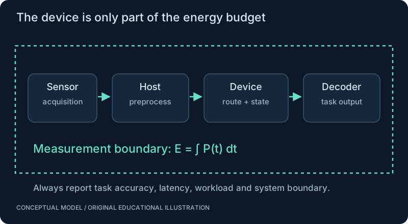
Estimate the full pipeline: sensor, preprocessing, network state, decoder and communication. Compare a simple baseline at the same required accuracy and deadline. A low-power network that requires a power-hungry host can lose the system-level comparison. A use-case sheet should be allowed to conclude that an SNN is not justified.
SEE THE RELATIONSHIPS
From structure to behavior.
MAKE THE IDEA PRECISE
The mathematics.
| Symbol | Meaning |
|---|---|
| usable_energy_Wh | Available energy within the chosen operating assumptions, watt-hours |
| average_power_W | Average whole-system power, watts |
| runtime_hours | Idealized operating duration, hours |
Build the equation, step by step
- Use energy actually available to the system, not just a nominal battery label. Keep the energy and power units compatible.
- Divide watt-hours by watts to obtain hours. The calculation assumes representative average power over the discharge interval.
- Include sensors, communication, processing and actuators in the boundary relevant to the task. Power changes with workload and operating conditions, so the quotient is an estimate rather than a guaranteed runtime.
WORK THROUGH THE NUMBERS
Worked example
An illustrative usable energy budget of 20 Wh and average consumption of 5 W gives 4 hours. Conversion loss, battery behavior and changing workload can reduce real runtime.
A small Python experiment.
Python 3 · Standard library only · Synthetic educational example. Run this in your own notebook or a local file.
usable_wh, average_w = 20.0, 5.0
print(f"idealized runtime = {usable_wh/average_w:.1f} h")
Expected output
idealized runtime = 4.0 h
Change one quantity, predict the result, and then run the code again. Explain any difference before adding complexity.
Test your understanding.
Try it: Add 3 W of host and sensor overhead. How does the estimated operating duration change?
Self-check: Would an efficient neural chip necessarily extend a robot’s runtime substantially?
Not if motors or other components dominate consumption. Quantify the component budget first. A large reduction in a small component can produce only a small whole-system gain; extra sensors or host computation can cancel it.
Where this model stops: The atlas is a decision framework, not evidence that every listed application benefits from spiking computation.
A research question: Which task-specific constraint would justify paying the extra integration cost?
Record evidence in your mastery worksheet →THE NEXT LAYER
Chapter depth map.
This introduction provides a first model. The following chapters are outlines for deeper future editions; their full treatments have not yet been published.
Machines in physical environments
23.1 Mobile platforms · Outline
- 23.1.1 Micro-drones and autonomous drones
- 23.1.2 Rovers, planetary rovers and autonomous vehicles
- 23.1.3 Humanoids and search-and-rescue robots
- 23.1.4 Agricultural, underwater and space robotics
- 23.1.5 Navigation, collision avoidance and sensor constraints
23.2 Work and infrastructure · Outline
- 23.2.1 Robot arms, warehouse robots and factory robots
- 23.2.2 Motion detection and industrial monitoring
- 23.2.3 Event-based surveillance and smart cameras
- 23.2.4 Swarm robotics and distributed sensing
- 23.2.5 Privacy, environmental variation and deployment constraints
Edge and human-facing applications
23.3 Low-power and adaptive devices · Outline
- 23.3.1 Low-power edge AI and always-on sensing
- 23.3.2 Wearables and adaptive sensors
- 23.3.3 Prosthetics and brain-machine interfaces
- 23.3.4 Clinical translation is a separate validated process
- 23.3.5 Conventional alternatives before biological analogies
23.4 The use-case decision sheet · Outline
- 23.4.1 Problem, sensors, architecture and models
- 23.4.2 Hardware, software and operating environment
- 23.4.3 Derive latency and power budgets from task needs
- 23.4.4 Limitations, fallback and conventional baseline
- 23.4.5 Explicit SNN/connectome justification or rejection
Read with the original sources.
These readings support the concepts and deeper investigation. The worked numbers and illustrations above are teaching examples.
Author manuscript / survey
Gallego et al.: Event-based Vision, A Survey ↗
A field map for sensing, representations and algorithms. Follow its cited primary experiments before asserting an application advantage.
Official hardware research resource
Intel — neuromorphic computing research ↗
Study event processing, memory and mapping constraints. Do not assume public hardware access or transfer platform-specific energy claims to a new task.