What you will learn
Simulate a closed-loop rover with bounded commands, state estimates, and documented failure conditions.
Before you begin: Foundations: matter, mathematics & computation; From neurons to brains
A robot acts on an uncertain estimate
A controller usually receives estimates, not perfect physical state. A camera, IMU or encoder has its own frame, timestamp, noise and calibration. A correct number in the wrong coordinate frame can be a wrong command. Write the frame and unit of every quantity before connecting a neural output to a controller.
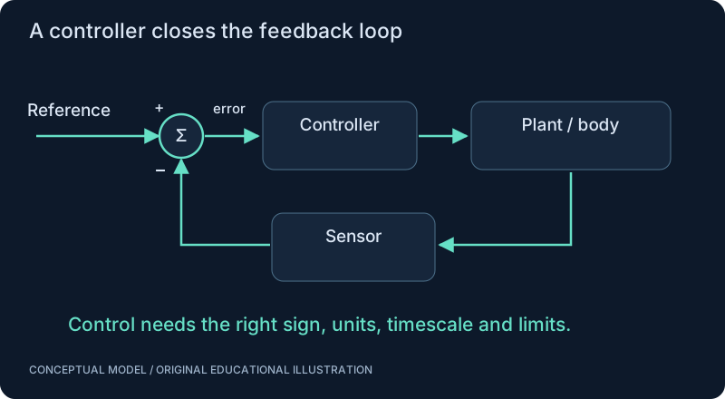
Feedback makes errors visible
Compare a target with the measured state to obtain an error. Proportional feedback responds to the present error, integral action accumulates persistent error, and derivative action responds to change. Real systems add saturation, delays, noise and actuator dynamics. A proportional controller for an ideal position integrator is a teaching example, not a tuning recipe for every robot.
Neural-network perspective
Perception can estimate obstacles, motion or state, while a separate control loop stabilizes the machine. An SNN might supply a reflex signal or learned feature. Its output must still have a meaning in the controller’s coordinate system and time budget. Evaluate what happens when perception becomes stale or uncertain.
Close the loop in simulation
Use a simple plant first. Record target, estimate, error, command and resulting state for each step. Test wrong signs, noisy sensors and saturation deliberately. A successful nominal trajectory is weaker evidence than a repeatable set of disturbance and recovery tests.
SEE THE RELATIONSHIPS
From structure to behavior.
MAKE THE IDEA PRECISE
The mathematics.
| Symbol | Meaning |
|---|---|
| x, x_target | Actual and desired position, meters |
| e | Position error, meters |
| Kp | Gain, inverse seconds for this velocity-input model |
| u | Commanded velocity, meters per second |
| dt | Step duration, seconds |
Build the equation, step by step
- Define error as target minus current position. A positive proportional gain then commands motion toward a fixed target in this ideal model.
- Treat u as a velocity command and multiply by dt to get a position increment. If u were acceleration or motor torque, the plant equation would be different.
- Substitute the controller into the update. For a fixed target, next error is (1 − dt Kp) times current error. This ideal scalar model converges when 0 < dt Kp < 2; real delays and dynamics change that condition.
WORK THROUGH THE NUMBERS
Worked example
Starting at 0 m with a 1 m target, Kp = 2 per second and dt = 0.1 s, the first command is 2 m/s and the state becomes 0.2 m. The next state becomes 0.36 m as the error decreases.
A small Python experiment.
Python 3 · Standard library only · Synthetic educational example. Run this in your own notebook or a local file.
x, target, gain, dt = 0.0, 1.0, 2.0, 0.1
for _ in range(2):
    velocity = gain*(target-x)
    x += dt*velocity
    print(f"{x:.2f} m")
Expected output
0.20 m
0.36 m
Change one quantity, predict the result, and then run the code again. Explain any difference before adding complexity.
Test your understanding.
Try it: Try dt times Kp greater than 2. Explain the resulting behavior before adding saturation.
Self-check: Why is the same gain not automatically valid at a new update rate?
The effective discrete correction depends on dt Kp. Changing the time step changes how strongly each update acts and can introduce oscillation or instability. A real robot also has delays, saturation and dynamics absent from this example.
Where this model stops: The ideal plant ignores inertia, sensor lag and actuator bounds. Its stability analysis does not transfer directly to physical hardware.
A research question: Does the neural layer improve performance when sensing delay and uncertainty are matched?
Record evidence in your mastery worksheet →THE NEXT LAYER
Chapter depth map.
This introduction provides a first model. The following chapters are outlines for deeper future editions; their full treatments have not yet been published.
Geometry and dynamics
13.1 Where is the robot? · Outline
- 13.1.1 Coordinate systems and frame transforms
- 13.1.2 Rotation matrices and orientation conventions
- 13.1.3 Forward and inverse kinematics
- 13.1.4 Dynamics, forces and inertia
- 13.1.5 Units, timestamps and sensor extrinsics
13.2 Control and estimation · Outline
- 13.2.1 Feedback control and stability
- 13.2.2 PID, saturation and integral windup
- 13.2.3 State-space models and Kalman filters
- 13.2.4 IMU bias, sensor fusion and observability
- 13.2.5 Optical flow and uncertainty propagation
Perception to motion
13.3 Navigation systems · Outline
- 13.3.1 SLAM and map uncertainty
- 13.3.2 Planning and collision checking
- 13.3.3 Trajectory generation and tracking
- 13.3.4 Sensor dropouts and recovery
- 13.3.5 ROS 2 concepts as an optional integration layer
13.4 A neural controller interface · Outline
- 13.4.1 Camera to SNN to activity decoder
- 13.4.2 Descending-neuron-like output as an analogy
- 13.4.3 Command bounds, rate limits and watchdogs
- 13.4.4 Separate learned decisions from stabilization
- 13.4.5 Simulation comparisons with classical control
Read with the original sources.
These readings support the concepts and deeper investigation. The worked numbers and illustrations above are teaching examples.
Official engineering documentation
PX4 — official simulation guide ↗
Begin with simulation and versioned interfaces. Simulation success alone does not establish hardware flight readiness.
Author-hosted engineering textbook
Lynch & Park — Modern Robotics, feedback control ↗
Reference for control concepts. Our scalar examples are teaching models, not robot-ready control implementations.