What you will learn
Turn an attractive idea into a preregistered comparison with realistic failure outcomes.
Before you begin: AGI connections: evidence before promises; Connectome programming
Make the frontier specific
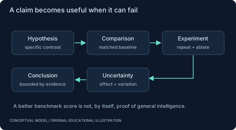
A promising question has a variable you can manipulate, a result you can measure and a baseline that could win. Asking whether biological connectivity helps is too broad. Asking whether a fixed topology reduces sample requirements for a bounded navigation task under matched degree and compute constraints is testable.
Separate the causal candidates
Topology, weight distribution, dynamics, encoder and decoder can all affect behavior. Changing several at once prevents a clean conclusion about any one. Use an ablation matrix and reserve evaluation cases before tuning. Parameter sensitivity matters when a connectome does not supply the dynamics you need.
Neural-network perspective
A biological motif can be treated as an inductive-bias candidate alongside generic sparsity, recurrence or modularity. The scientific value of a comparison includes negative results. If a simpler network matches the result, the study can clarify which complexity is unnecessary rather than hide the comparison.
SEE THE RELATIONSHIPS
From structure to behavior.
MAKE THE IDEA PRECISE
The mathematics.
| Symbol | Meaning |
|---|---|
| delta_i | Paired candidate-minus-baseline score for independent run i |
| n | Number of paired runs |
| SE | Estimated standard error of the mean under independence assumptions |
Build the equation, step by step
- Pair candidate and baseline measurements under matched conditions and compute their differences.
- Average those differences for the estimated effect. Estimate sample standard deviation using n − 1 in the variance denominator, requiring at least two pairs.
- For independent comparable pairs, estimated standard error of the mean is sample standard deviation divided by the square root of n. Correlated trials, selection after looking at results and dataset leakage can invalidate a naive interpretation.
WORK THROUGH THE NUMBERS
Worked example
Illustrative paired differences [0.04, 0.02, -0.01, 0.03] have mean 0.020 and estimated standard error about 0.011. Four runs are a small example, not an adequate universal experimental sample size.
A small Python experiment.
Python 3 · Standard library only · Synthetic educational example. Run this in your own notebook or a local file.
from statistics import mean, stdev
from math import sqrt
differences = [0.04, 0.02, -0.01, 0.03]
print(f"mean = {mean(differences):.3f}; SE = {stdev(differences)/sqrt(len(differences)):.3f}")
Expected output
mean = 0.020; SE = 0.011
Change one quantity, predict the result, and then run the code again. Explain any difference before adding complexity.
Test your understanding.
Try it: Compare independent evaluation environments with repeated measurements from the same trajectory.
Self-check: Is one standard error a 95% confidence interval?
No. It is an estimated scale of uncertainty for the mean under assumptions. A confidence interval needs an appropriate multiplier and distributional method; small samples commonly require different treatment from a large-sample normal approximation. Neither interval alone establishes practical importance.
Where this model stops: A standard error is not a confidence interval or a proof of causality.
A research question: Which conclusions remain stable under rewiring, parameter sweeps and changed task distributions?
Record evidence in your mastery worksheet →THE NEXT LAYER
Chapter depth map.
This introduction provides a first model. The following chapters are outlines for deeper future editions; their full treatments have not yet been published.
Architecture and learning
22.1 Structure as an inductive bias · Outline
- 22.1.1 Connectome-inspired architectures and matched controls
- 22.1.2 Circuit motifs versus generic sparsity
- 22.1.3 Training data requirements and sample efficiency
- 22.1.4 Specialized circuits emerging through learning
- 22.1.5 Transformers combined with structural priors
22.2 Timing and adaptation · Outline
- 22.2.1 Local biological learning rules at scale
- 22.2.2 Neuromodulators and missing receptor information
- 22.2.3 Architecture versus learned dynamics
- 22.2.4 Robustness to unknown delays and synaptic strengths
- 22.2.5 Compare rate and temporal representations
Embodied and efficient intelligence
22.3 Physical hypotheses · Outline
- 22.3.1 World models communicating with reflex SNNs
- 22.3.2 Always-on neuromorphic robots
- 22.3.3 Body/environment contributions to behavior
- 22.3.4 Whole-system energy versus kernel efficiency
- 22.3.5 Cases where simpler controllers are sufficient
22.4 A falsifiable proposal · Outline
- 22.4.1 Primary outcome and effect-size target
- 22.4.2 Baseline and ablation matrix
- 22.4.3 Compute and data budget
- 22.4.4 Replication and sensitivity analysis
- 22.4.5 Negative results, stopping criteria and open questions
Read with the original sources.
These readings support the concepts and deeper investigation. The worked numbers and illustrations above are teaching examples.
Primary paper
Shiu et al. (2024): a Drosophila computational brain model ↗
A connectome-based computational model of sensorimotor processing. Separate experimentally tested predictions from the model assumptions and untested behaviors.
Primary paper
Lin et al. (2024): network statistics of the fly connectome ↗
Study motif and network analysis with attention to filtering and null-model choices. Graph centrality is not automatically causal importance.
Official hardware research resource
Intel — neuromorphic computing research ↗
Study event processing, memory and mapping constraints. Do not assume public hardware access or transfer platform-specific energy claims to a new task.