Connectome programming

What you will learn

Build a small audited subgraph, preserve metadata, and test its conversion into a sparse simulator.

Before you begin: Connectomics: wiring as data; Computational neuroscience; Spiking neural networks

A data pipeline is part of the experiment

A reliable pipeline records the dataset, release, neuron-selection query, edge filters and annotation provenance. Official MaleCNS downloads and neuPrint resources provide paths into versioned data, but access details and schemas can change. This website does not fetch a private token or query a live connectome database. The lesson uses synthetic records so that its behavior is completely inspectable.

Identifiers are not array indices

Real identifiers can be sparse, large and specific to a dataset. Build an explicit mapping from external IDs to compact internal indices. Preserve the reverse mapping for interpretation. When filtering neurons, specify what happens to connections whose targets fall outside the selected set; silent omission can change the modeled boundary conditions.

Neural-network perspective

An edge list becomes neural connectivity only after you choose orientation, weight units, dynamics, delays and input/output mappings. Synapse counts can be a structural prior, but a model must not present them as measured physiological weights. Store every transformation in a manifest so that an alternative mapping can be tested.

Scale by profiling

For a sparse network, storing only edges can avoid a quadratic dense matrix. Yet irregular memory access and event routing can dominate runtime. First build a small correct conversion, then profile memory and processing cost before choosing NetworkX, sparse arrays or a learning framework.

SEE THE RELATIONSHIPS

From structure to behavior.

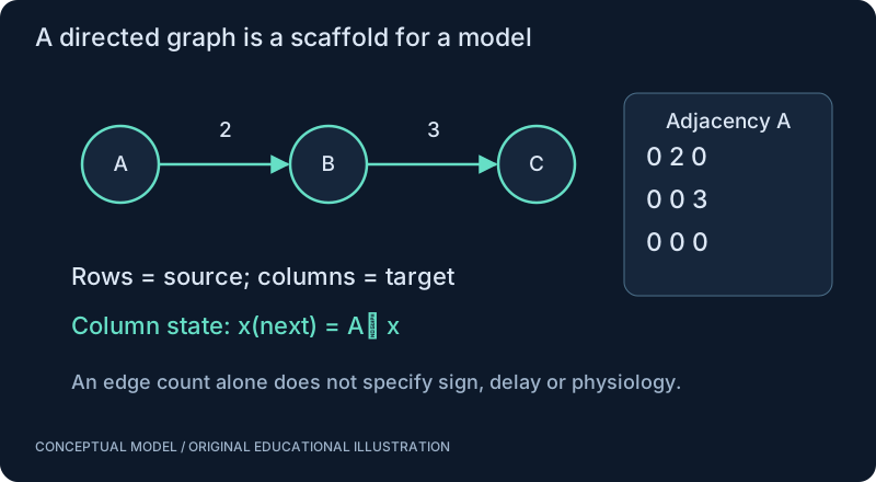
Connectome: a labelled conceptual diagram — Figure 11.1 · Connectome. Original educational diagram; synthetic, not a measured result.

A learning flow for this part. Follow the assumptions through to an observable result.

MAKE THE IDEA PRECISE

The mathematics.

dense entries = N²; edge-list records = M

Symbols and units
Symbol	Meaning
N	Number of selected neurons
M	Number of retained directed edges
N²	All possible source-target pairs, including absent connections

Build the equation, step by step

For N indexed nodes, a dense directed matrix has N rows and N columns, hence N squared entries including possible self-connections.
An edge list stores M records. Each record needs source, target and whatever fields the model requires; its byte cost is not merely the weight size.
Map persistent external identifiers to contiguous local indices with a reversible lookup. Sorting or filtering must not silently change the association between edges and state vectors.

WORK THROUGH THE NUMBERS

Worked example

Three external IDs map to positions 0, 1 and 2. Two retained edges are translated through that mapping. The demonstration keeps a count field unchanged and makes no physiological weighting claim.

A small Python experiment.

Python 3 · Standard library only · Synthetic educational example. Run this in your own notebook or a local file.

ids = [101, 9001, 42]
index = {neuron:i for i,neuron in enumerate(ids)}
edges = [(101, 42, 3), (42, 9001, 2)]
compact = [(index[a],index[b],count) for a,b,count in edges]
print(compact)

Expected output

[(0, 2, 3), (2, 1, 2)]

Change one quantity, predict the result, and then run the code again. Explain any difference before adding complexity.

Test your understanding.

Try it: Add an edge to an ID outside the selection. Decide whether to reject it, drop it with a log, or expand the selection.

Self-check: Why should an identifier such as 9001 not become array position 9001?

Identifiers may be sparse, very large, noncontiguous or version-specific. Direct indexing wastes space and can mix datasets. Keep a mapping and its inverse, validate endpoints, and record the dataset version that gives those IDs meaning.

Where this model stops: Synthetic IDs here are not real biological annotations. Large-data access and full simulation remain separate experiments.

A research question: How does the chosen subgraph boundary alter spontaneous and driven activity?

Record evidence in your mastery worksheet →

THE NEXT LAYER

Chapter depth map.

This introduction provides a first model. The following chapters are outlines for deeper future editions; their full treatments have not yet been published.

From query to graph

11.1 Data access and identity · Outline

11.1.1 neuPrint and documented query interfaces
11.1.2 FlyWire tools and MaleCNS exports
11.1.3 Neuron IDs, cell types and region filters
11.1.4 Synapse queries, pagination and access conditions
11.1.5 Pin release, query, license and downloaded-file hash

11.2 Conversion without silent assumptions · Outline

11.2.1 Typed edge lists and duplicate handling
11.2.2 NetworkX graphs for exploration
11.2.3 Sparse adjacency matrices with verified orientation
11.2.4 PyTorch tensors and index remapping
11.2.5 Count-to-weight choices and uncertainty

From graph to experiment

11.3 Assigning dynamics · Outline

11.3.1 Neuron-model parameters are extra assumptions
11.3.2 Excitatory/inhibitory interpretation needs receptor context
11.3.3 Input mapping, delays and initial conditions
11.3.4 Subgraph boundary treatment and missing inputs
11.3.5 Validate small examples before large exports

11.4 Large sparse data · Outline

11.4.1 Streaming reads and chunked queries
11.4.2 Sparse matrix formats and memory budgets
11.4.3 Vectorization, event updates and profiling
11.4.4 Reproducible graph-to-simulation manifests
11.4.5 Activity analysis and sensitivity experiments

Read with the original sources.

These readings support the concepts and deeper investigation. The worked numbers and illustrations above are teaching examples.

Official dataset tool