Computational neuroscience

What you will learn

Implement and test LIF dynamics, then explain what richer models add and what they cost.

Before you begin: Biological neuroscience; Foundations: matter, mathematics & computation

Choose the model by the question

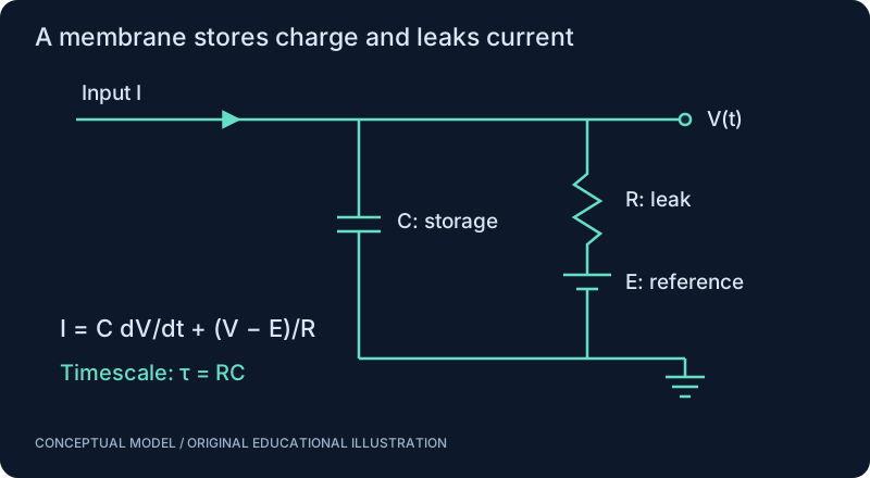
A McCulloch–Pitts unit describes a thresholded combination of inputs without membrane dynamics. An integrate-and-fire model introduces accumulation; adding leakage produces LIF. Izhikevich models add recovery dynamics, while Hodgkin–Huxley models represent voltage-dependent conductances. More equations are useful only when their parameters and mechanisms help answer the question being tested.

Turn a derivative into an update

A derivative describes change per unit time. Forward Euler approximates the next state by adding the current slope times a small interval. For LIF, compute the leak and input terms, scale by dt/tau, then apply your threshold/reset convention. Spike detection and refractory handling are additional rules: the differential equation alone does not define them.

Check against something known

Before running a network, test a neuron below threshold where a constant-current solution is available. Halve the timestep and compare the voltage trajectory. Then test reset and refractory behavior independently. A simulation that looks smooth may still have inconsistent units or an off-by-one delay. The interactive figure below is an illustrative current-driven LIF cell, not fitted biological data.

Interpret the network perspective

An evolving membrane variable is a temporal feature accumulator. Its output spike can drive downstream states. Scaling to thousands of cells requires decisions about sparse connectivity, synaptic filtering, delay queues and random-number generation. Start with an inspectable numerical reference so that speedups can be tested for semantic changes.

SEE THE RELATIONSHIPS

From structure to behavior.

Membrane: a labelled conceptual diagram — Figure 6.1 · Membrane. Original educational diagram; synthetic, not a measured result.

Spike train: a labelled conceptual diagram — Figure 6.2 · Spike train. Original educational diagram; synthetic, not a measured result.

A learning flow for this part. Follow the assumptions through to an observable result.

CHANGE A PARAMETER. TEST YOUR INTUITION.

A neuron as a leaky integrator

Hold current constant for 200 ms. The voltage leaks toward rest, rises with input, and resets after a threshold crossing. Values are a toy model, not fitted biology.

R = 100 MΩ; rest/reset = −65 mV; threshold = −50 mV; refractory period = 2 ms; Euler step = 0.1 ms. A threshold crossing is counted as a spike, without modelling its biological waveform.

Interactive controls load with JavaScript. The worked example below is available without it.

MAKE THE IDEA PRECISE

The mathematics.

V_next = V + (dt / tau) [-(V - E) + R I]

Symbols and units
Symbol	Meaning
V, V_next	Current and next membrane potential, mV
dt, tau	Timestep and membrane time constant, ms
E	Leak reference potential, mV
R	Resistance, megaohms
I	Input current, nanoamps; R I is mV

Build the equation, step by step

Begin with τ dV/dt = −(V − E) + RI. The leak term pulls voltage toward E; the input term shifts the equilibrium to E + RI.
Approximate dV/dt by (V_next − V)/dt, evaluate the right-hand side at the old voltage, and solve for V_next. This produces the explicit Euler update.
Threshold and reset are additional rules, not consequences of that linear differential equation. For constant suprathreshold input, the first crossing time from E is −τ ln(1 − (V_threshold − E)/(RI)); this gives a numerical reference check.

WORK THROUGH THE NUMBERS

Worked example

For V = E = -65 mV, tau = 20 ms, dt = 1 ms, R = 100 megaohms and I = 0.2 nA, the first update is -64 mV. That is a numerical subthreshold step, not a full action-potential waveform.

A small Python experiment.

Python 3 · Standard library only · Synthetic educational example. Run this in your own notebook or a local file.

V = E = -65.0
tau, dt, R, I = 20.0, 1.0, 100.0, 0.2
V_next = V + dt/tau * (-(V-E) + R*I)
print(f"next voltage = {V_next:.1f} mV")

Expected output

next voltage = -64.0 mV

Change one quantity, predict the result, and then run the code again. Explain any difference before adding complexity.

Test your understanding.

Try it: Compute the second step by hand. Then halve dt while keeping total simulated time fixed.

Self-check: What happens if the time step is too large?

An explicit update can miss threshold timing and distort decay; sufficiently large steps can become unstable even when the continuous model is stable. Compare results after halving dt, and test a passive subthreshold trace against its analytic exponential solution before trusting spike counts.

Where this model stops: LIF omits detailed channel and dendritic dynamics. A one-step example does not establish numerical convergence.

A research question: Which behavior changes when you replace fixed-current synapses with conductance-based ones?

Record evidence in your mastery worksheet →

THE NEXT LAYER

Chapter depth map.

This introduction provides a first model. The following chapters are outlines for deeper future editions; their full treatments have not yet been published.

From idealized units to dynamical neurons

6.1 Threshold units and integrators · Outline

6.1.1 McCulloch-Pitts logic and its biological limits
6.1.2 Integrate-and-fire state and threshold
6.1.3 Derive tau_m dV/dt = -(V - V_rest) + R I(t)
6.1.4 Meaning and units of every parameter
6.1.5 Constant-current solution and a worked voltage update

6.2 A reliable LIF simulator · Outline

6.2.1 Euler steps and analytic subthreshold comparison
6.2.2 Spike detection, reset and refractory periods
6.2.3 Synaptic currents, delays and noise
6.2.4 Timestep refinement and event-order conventions
6.2.5 Voltage traces, spike rasters and firing-rate curves

Model fidelity and scale

6.3 Beyond LIF · Outline

6.3.1 Izhikevich recovery variable and reset dynamics
6.3.2 Hodgkin-Huxley conductance and gating variables
6.3.3 Conductance-based synapses and reversal potentials
6.3.4 Parameter fitting and identifiability
6.3.5 Match model complexity to measurements

6.4 Simulating networks · Outline

6.4.1 One, ten, one hundred and one thousand cells
6.4.2 Sparse connectivity and event queues
6.4.3 Reproducibility, seeds and deterministic comparisons
6.4.4 Memory and throughput estimates for larger networks
6.4.5 Brian2 and NEST as tools to evaluate after the baseline

Read with the original sources.

These readings support the concepts and deeper investigation. The worked numbers and illustrations above are teaching examples.

Author-hosted textbook