Spiking neural networks

What you will learn

Train or adapt a small SNN and compare it with a matched non-spiking baseline.

Before you begin: Computational neuroscience; From neurons to brains

Represent both activity and time

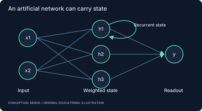
An ordinary feedforward layer maps an input vector to an output vector. A spiking layer also keeps state: a membrane value, possibly synaptic current and a refractory timer. An output event occurs according to a threshold rule. This is a computational representation, not an assertion that every artificial spike reproduces every property of a biological action potential.

A learning problem appears at the threshold

The hard threshold is discontinuous. Surrogate-gradient methods keep a spiking forward computation but use a convenient smooth approximation in the backward calculation. That is a deliberate estimator choice. Local plasticity rules such as STDP operate differently; reward modulation introduces a further credit-assignment mechanism. Compare what information each rule requires.

Encoding can dominate the result

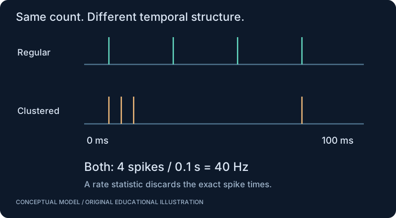
Converting a static value to many spikes costs time and operations. A low firing rate is not automatically efficient if you require a long window to recover the answer. Compare rate, latency and population representations under the same task deadline. Count encoder, decoder, host and communication overhead when interpreting a power claim.

A small network first

The recurrent update below is a subthreshold teaching abstraction with dimensionless quantities. It shows state retention and a weighted event input without claiming to be a full SNN implementation. Add thresholds only after you can explain where each input is routed. A network diagram should show temporal state as well as connection lines.

SEE THE RELATIONSHIPS

From structure to behavior.

Network: a labelled conceptual diagram — Figure 7.1 · Network. Original educational diagram; synthetic, not a measured result.

Spike train: a labelled conceptual diagram — Figure 7.2 · Spike train. Original educational diagram; synthetic, not a measured result.

A learning flow for this part. Follow the assumptions through to an observable result.

MAKE THE IDEA PRECISE

The mathematics.

u_next = beta u + W s

Symbols and units
Symbol	Meaning
u	Membrane-state vector in an illustrative discrete model
beta	Retention factor between zero and one
W	Weight matrix with target rows and source columns here
s	Binary source spike vector

Build the equation, step by step

Represent each presynaptic spike in the current bin by a vector entry. Decide whether an entry is binary or a count and keep that convention explicit.
Multiply W by the spike vector to sum contributions to each target. Here W stores targets in rows, unlike the source-row adjacency used in the connectomics part.
Add the decayed previous state βu. For an exact passive decay over a bin, β = exp(−dt/τ); a full spiking model still needs explicit threshold, reset and timing conventions.

WORK THROUGH THE NUMBERS

Worked example

For u = [0.2, 0.4], beta = 0.9, s = [1, 0], and W rows [0.5, -0.1], [0.2, 0.3], the new state is [0.68, 0.56]. Notice that the matrix convention differs from the graph example; declare it explicitly.

A small Python experiment.

Python 3 · Standard library only · Synthetic educational example. Run this in your own notebook or a local file.

u, s = [0.2, 0.4], [1, 0]
W = [[0.5, -0.1], [0.2, 0.3]]
v = [0.9*u[j] + sum(w*x for w,x in zip(row,s)) for j,row in enumerate(W)]
print([round(x, 2) for x in v])

Expected output

[0.68, 0.56]

Change one quantity, predict the result, and then run the code again. Explain any difference before adding complexity.

Test your understanding.

Try it: Set both input spikes to zero and trace state decay for five steps.

Self-check: Why can swapping a matrix transpose silently break a neural simulation?

Both orientations may have compatible shapes in a square network, so the code runs while reversing connection direction. Test a tiny asymmetric graph with a single active source and a hand-calculated expected target before scaling up.

Where this model stops: Neither sparsity nor biological resemblance guarantees accuracy, energy savings or general intelligence.

A research question: Does timing preserve useful information that a matched rate baseline loses?

Record evidence in your mastery worksheet →

THE NEXT LAYER

Chapter depth map.

This introduction provides a first model. The following chapters are outlines for deeper future editions; their full treatments have not yet been published.

Representation and inference

7.1 ANNs, CNNs, RNNs, Transformers and SNNs · Outline

7.1.1 Activation values versus discrete events
7.1.2 Membrane states and temporal recurrence
7.1.3 Spatial convolution, recurrent state and attention
7.1.4 Latency, memory and operation-count tradeoffs
7.1.5 Why spikes do not guarantee energy savings
7.1.6 Conventional learning primer: losses, supervised learning, training/validation splits and optimization

7.2 Encoding and decoding · Outline

7.2.1 Rate, latency and temporal encodings
7.2.2 Population codes and event-based input
7.2.3 Spike counts, first-spike and filtered-rate decoding
7.2.4 Input scaling, clipping and observation windows
7.2.5 Encode-decode tests with known synthetic signals

Learning and large sparse systems

7.3 Learning with discontinuous spikes · Outline

7.3.1 Backpropagation through time and state unrolling
7.3.2 Surrogate gradients and estimator bias
7.3.3 Hebbian rules, STDP and local learning
7.3.4 Reward-modulated STDP and eligibility traces
7.3.5 Homeostasis and stability during learning

7.4 Implement, profile and compare · Outline

7.4.1 Pure Python baseline before framework abstraction
7.4.2 PyTorch-oriented Norse and snnTorch options
7.4.3 Dense versus sparse updates at different spike rates
7.4.4 Scaling from 1 to 1000 cells and beyond
7.4.5 Fair accuracy, latency, energy and robustness benchmarks

Read with the original sources.

These readings support the concepts and deeper investigation. The worked numbers and illustrations above are teaching examples.

Research tutorial / author manuscript