What you will learn
Build controlled motion stimuli and separate direction, expansion, and brightness responses.
Before you begin: Drosophila: anatomy, circuits & datasets; Computational neuroscience
Geometry arrives before interpretation
An approaching object occupies an increasing visual angle. A motion-sensitive system must distinguish that expansion from translation, brightness changes and self-motion. A camera does not directly observe distance; the image combines scene geometry, motion and optical projection. Make those assumptions explicit before converting pixels into an action.
Useful circuits, careful claims
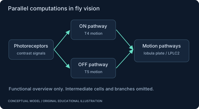
T4/T5 direction-selective responses and LPLC2 looming selectivity are experimentally studied cases, not a universal visual algorithm. Their relevance here is methodological: define a stimulus, measure a response, test alternative stimuli, and relate the result to circuitry. The branching diagram is a functional orientation, not a synapse-resolved reconstruction.
An engineered looming proxy
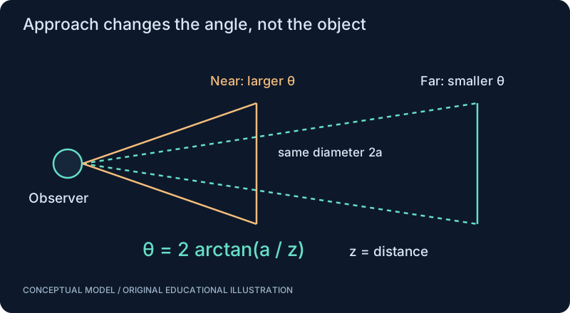
For a centered circular object of radius a at distance z in a simple pinhole geometry, its angular diameter is 2 atan(a/z). Under straight constant-speed approach, its derivative grows as the object comes nearer. Time-to-contact estimates require additional motion assumptions; a turning or expanding object can break them. A detector should be evaluated on these confounders.
Neural-network perspective
Local temporal filters can provide motion features. Pooling those features with spatial direction preferences creates an expansion-sensitive hypothesis. Compare it against a conventional optical-flow or frame-difference detector before attributing an advantage to spikes. Evaluate false alarms and reaction time, not only visually convincing demonstrations.
SEE THE RELATIONSHIPS
From structure to behavior.
CHANGE A PARAMETER. TEST YOUR INTUITION.
Why a nearby object looms larger
Move an object with radius 0.1 m closer. The angular size changes nonlinearly; this display is geometry, not a simulation of the fly's neurons.
Interactive controls load with JavaScript. The worked example below is available without it.
MAKE THE IDEA PRECISE
The mathematics.
| Symbol | Meaning |
|---|---|
| theta | Angular diameter, radians |
| a | Object radius, meters |
| z | Distance along the camera axis, meters |
| atan | Inverse tangent |
Build the equation, step by step
- Draw a line from the observer to the object centre and another to its edge. The right triangle has opposite side a and adjacent side z.
- The half-angle satisfies tan(θ/2) = a/z. Apply the inverse tangent and double the result to get angular diameter.
- Radians are the natural mathematical unit. Convert to degrees only for display. When a/z is small, θ is approximately 2a/z radians; the approximation degrades for nearby large objects.
WORK THROUGH THE NUMBERS
Worked example
An object of radius 0.5 m at 5 m subtends approximately 11.42 degrees. At 2.5 m it subtends approximately 22.62 degrees. Angular growth is nonlinear; doubling apparent angle is only approximately related to halving distance at small angles.
A small Python experiment.
Python 3 · Standard library only · Synthetic educational example. Run this in your own notebook or a local file.
from math import atan, degrees
a = 0.5
for z in [5.0, 2.5]:
    print(f"{degrees(2*atan(a/z)):.2f} degrees")
Expected output
11.42 degrees
22.62 degrees
Change one quantity, predict the result, and then run the code again. Explain any difference before adding complexity.
Test your understanding.
Try it: Keep distance fixed and increase physical radius. Explain why expansion is not proof of approach.
Self-check: Can angular size alone reveal distance?
Not without information about physical size or another cue. A small nearby object and a larger distant object can subtend the same angle. Changes over time provide additional information, but require assumptions about object shape and relative motion.
Where this model stops: Angular size alone does not determine depth or collision risk.
A research question: Can an expansion detector reject self-rotation and illumination changes without excessive delay?
Record evidence in your mastery worksheet →THE NEXT LAYER
Chapter depth map.
This introduction provides a first model. The following chapters are outlines for deeper future editions; their full treatments have not yet been published.
From light to motion
8.1 Signals before objects · Outline
- 8.1.1 Photons and photoreceptor transduction
- 8.1.2 Local contrast and adaptation
- 8.1.3 Spatial sampling and temporal filtering
- 8.1.4 ON and OFF information
- 8.1.5 Compare the fly visual front end with engineered cameras
8.2 Direction-selective circuits · Outline
- 8.2.1 Delayed correlation and motion-energy intuition
- 8.2.2 T4/T5 tuning and pathway distinctions
- 8.2.3 Optic flow from self-motion and object motion
- 8.2.4 Aperture ambiguity and contrast dependence
- 8.2.5 Compare circuit models with optical flow and CNNs
Approach, escape and evaluation
8.3 Looming as geometry and computation · Outline
- 8.3.1 Angular size and expansion rate
- 8.3.2 Time-to-contact under explicit motion assumptions
- 8.3.3 LPLC2 and radial motion opponency
- 8.3.4 Distinguish looming, translation and luminance change
- 8.3.5 Circuit evidence versus an engineered detector
8.4 From visual signal to reflex · Outline
- 8.4.1 Visual projection and descending pathways
- 8.4.2 Escape and collision-avoidance hypotheses
- 8.4.3 Stimulus sweeps and negative controls
- 8.4.4 Noise, occlusion and background motion
- 8.4.5 Evaluate robotics relevance in simulation
Read with the original sources.
These readings support the concepts and deeper investigation. The worked numbers and illustrations above are teaching examples.
Primary paper
Maisak et al. (2013): a directional tuning map ↗
Experimental work on direction-selective T4/T5 populations and ON/OFF motion. Ask how tuning was measured and what the measurements do not establish.
Primary paper
Klapoetke et al. (2017): radial motion opponency ↗
A study of LPLC2 looming selectivity. Compare outward expansion with translation, contraction, and brightness controls.