What you will learn
Train a small predictive model and identify where rollout errors invalidate its plans.
Before you begin: Reinforcement learning + SNNs; Memory: biological & artificial
Predict before you act
A world model represents how some aspect of the environment may change. It might predict a physical state, an image or a latent representation. A useful prediction model is not necessarily a complete simulation of reality. Its value depends on whether its errors allow good decisions in the task you actually test.
Prediction error compounds
A one-step forecast can be accurate while a long imagined trajectory drifts far from reality. Feedback observations can correct estimates, while uncertainty can limit how far a planner trusts a rollout. Dreamer provides a research example of learned models used for imagined behavior learning; its results should be interpreted within the reported settings.
Biological theories need their own evidence
Predictive coding and active inference propose ways to understand aspects of perception and action. They should not be treated as interchangeable with every engineering world model, or as settled universal mechanisms. Read theoretical assumptions separately from experiments that test particular implementations.
Neural-network perspective
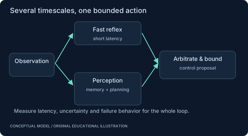
A recurrent or latent model can combine the current representation and an action to predict the next representation. An SNN reflex may operate alongside a slower model rather than waiting for a long forecast. Compare prediction quality, control outcomes and compute together; a visually convincing generated future may still be useless for control.
SEE THE RELATIONSHIPS
From structure to behavior.
MAKE THE IDEA PRECISE
The mathematics.
| Symbol | Meaning |
|---|---|
| x | Current scalar state |
| u | Action input |
| a, b | Chosen model coefficients |
| x_hat_next | Predicted next state |
| x_observed | Measured next state on the same scale |
Build the equation, step by step
- Use the current state and action to produce a next-state prediction. A scalar linear model assumes fixed coefficients and a simple state representation.
- Subtract prediction from the observed next state. Squaring removes the sign and emphasizes larger errors.
- For a position state, squared error has units of distance squared. Mixing position, angle and velocity errors in one loss requires explicit scaling. Good one-step error does not guarantee good long-horizon planning.
WORK THROUGH THE NUMBERS
Worked example
With x = 1, u = 0.2, a = 0.8 and b = 0.5, prediction is 0.9. An observed value of 1.1 produces error 0.2 and squared error 0.04. The coefficients are illustrative, not fitted data.
A small Python experiment.
Python 3 · Standard library only · Synthetic educational example. Run this in your own notebook or a local file.
prediction = 0.8*1.0 + 0.5*0.2
error = 1.1 - prediction
print(f"prediction = {prediction:.2f}; squared error = {error**2:.2f}")
Expected output
prediction = 0.90; squared error = 0.04
Change one quantity, predict the result, and then run the code again. Explain any difference before adding complexity.
Test your understanding.
Try it: Roll the model forward for ten steps without corrections. Explain how an incorrect coefficient can accumulate error.
Self-check: Why can a good predictor fail during planning?
The planner may choose actions outside the training distribution or exploit systematic prediction errors. Small errors can compound over many steps. Evaluate rollouts under the policy that will actually use the model, including uncertainty and constraint violations.
Where this model stops: Small average prediction error does not guarantee safe decisions on rare events.
A research question: When should a fast reactive controller override a model-based plan?
Record evidence in your mastery worksheet →THE NEXT LAYER
Chapter depth map.
This introduction provides a first model. The following chapters are outlines for deeper future editions; their full treatments have not yet been published.
Representing possible futures
18.1 State-space and latent models · Outline
- 18.1.1 Observed and hidden state
- 18.1.2 Transition and observation models
- 18.1.3 Latent representations and uncertainty
- 18.1.4 Multi-step prediction and distribution shift
- 18.1.5 Calibration and identifiability
18.2 Model-based reinforcement learning · Outline
- 18.2.1 Learned rollouts and imagined trajectories
- 18.2.2 Planning in latent state
- 18.2.3 Model bias and compounding error
- 18.2.4 Dreamer as a reading case study
- 18.2.5 Compare with model-free and classical baselines
Biological theories and engineering claims
18.3 Prediction in neuroscience · Outline
- 18.3.1 Internal models and sensorimotor prediction
- 18.3.2 Predictive processing and predictive coding
- 18.3.3 Active inference: assumptions and objectives
- 18.3.4 Distinguish theory, mechanism and experiment
- 18.3.5 Avoid treating a debated unifying theory as settled fact
18.4 World model meets reflex · Outline
- 18.4.1 Slow forecasts and fast reactive loops
- 18.4.2 Confidence thresholds for intervention
- 18.4.3 Memory and model updates
- 18.4.4 Counterfactual evaluation and ablations
- 18.4.5 Test benefit under unexpected obstacles
Read with the original sources.
These readings support the concepts and deeper investigation. The worked numbers and illustrations above are teaching examples.
Primary research / versioned manuscript
Hafner et al.: Mastering Diverse Domains through World Models ↗
Read after latent dynamics and actor-critic learning. Evaluate imagined rollouts, model errors, and the scope of reported task results.
Theory / review by its proponent
Friston (2010) — The free-energy principle: a unified brain theory? ↗
Read as a proposed theoretical framework, not a settled description of every brain computation.