What you will learn
Compare learned policies across matched architectures, seeds, and training budgets.
Before you begin: Foundations: matter, mathematics & computation; Spiking neural networks; Robotics: estimation, planning & control
Actions change future evidence
In supervised learning, labels usually arrive as part of a dataset. In reinforcement learning, a policy chooses actions that influence future observations and rewards. A Markov decision process is a mathematical description with states, actions, transitions and rewards. If an observation omits important state, memory or belief-state estimation may be needed.
Return is not the immediate reward
A decision can have delayed consequences. Discounted return combines rewards across time, with gamma controlling how strongly later rewards contribute. A value function predicts return under specified behavior. Policy gradients adjust action-selection parameters; actor-critic methods combine a policy with value estimation. PPO is one family of policy-optimization methods, not a guarantee of learning a robust controller.
A spiking policy is a modeling choice
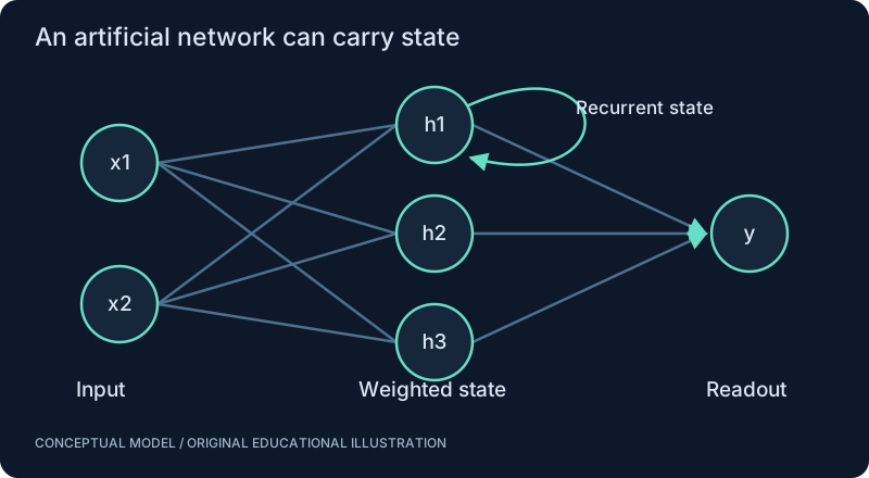
An SNN can encode observations, keep temporal state and produce activity for an action decoder. Compare it with a conventional recurrent policy under matching environment interactions, parameter budgets and evaluation seeds. If connectome structure is used, include degree-matched rewiring controls. Reward design and training data can explain success even when biological structure contributes little.
SEE THE RELATIONSHIPS
From structure to behavior.
MAKE THE IDEA PRECISE
The mathematics.
| Symbol | Meaning |
|---|---|
| G_0 | Discounted return beginning at time zero |
| r_t | Reward at step t |
| gamma | Discount factor between zero and one |
| t | Discrete decision step |
Build the equation, step by step
- Choose a reward convention and horizon. The reward at the first transition receives weight one, the next receives γ, and later rewards receive successive powers.
- Multiply each observed reward by its discount factor and add them to obtain a realized return.
- Expected value averages returns under a policy and environment distribution. One observed return is a sample, not the value function or evidence that a policy has learned.
WORK THROUGH THE NUMBERS
Worked example
Rewards [1, 0, 2] with gamma = 0.9 produce 1 + 0 + 1.62 = 2.62. Return depends on the chosen discount and reward definition, not on a universal meaning of success.
A small Python experiment.
Python 3 · Standard library only · Synthetic educational example. Run this in your own notebook or a local file.
rewards, gamma = [1, 0, 2], 0.9
value = sum((gamma**t)*r for t,r in enumerate(rewards))
print(f"return = {value:.2f}")
Expected output
return = 2.62
Change one quantity, predict the result, and then run the code again. Explain any difference before adding complexity.
Test your understanding.
Try it: Compare gamma = 0 and gamma = 1. Which behavior would each objective favor?
Self-check: If an agent gets a larger training return, is it better at the intended task?
Only if the reward captures the intended task and the comparison generalizes to held-out conditions. Reward exploits, changed termination rules and different budgets can make returns misleading. Keep a task-level evaluation separate from training feedback.
Where this model stops: Optimizing a reward can exploit loopholes or fail outside training conditions.
A research question: Does a structural prior improve sample efficiency after matching recurrence and compute?
Record evidence in your mastery worksheet →THE NEXT LAYER
Chapter depth map.
This introduction provides a first model. The following chapters are outlines for deeper future editions; their full treatments have not yet been published.
Learning from consequences
16.1 MDPs and value · Outline
- 16.1.1 States, actions, transitions and rewards
- 16.1.2 Markov assumptions and partial observability
- 16.1.3 Policies, returns and discounting
- 16.1.4 Value functions and Bellman equations
- 16.1.5 Q-learning and exploration
16.2 Policy optimization · Outline
- 16.2.1 Policy gradients and credit assignment
- 16.2.2 Actor-critic methods and variance reduction
- 16.2.3 PPO objective and clipping intuition
- 16.2.4 Reward design and unintended incentives
- 16.2.5 Evaluation seeds separate from training
Spiking and structural priors
16.3 Learning in a spiking policy · Outline
- 16.3.1 Temporal state and action decoding
- 16.3.2 Surrogate gradients versus local rules
- 16.3.3 Reward-modulated STDP and eligibility traces
- 16.3.4 Evolution strategies and neuroevolution
- 16.3.5 Cost of simulation and sample collection
16.4 Does connectome structure help? · Outline
- 16.4.1 Connectivity as an inductive-bias hypothesis
- 16.4.2 Degree-matched and randomly rewired controls
- 16.4.3 Fixed topology versus learned topology
- 16.4.4 Sample efficiency, robustness and compute
- 16.4.5 Reject the hypothesis if matched baselines win
Read with the original sources.
These readings support the concepts and deeper investigation. The worked numbers and illustrations above are teaching examples.
Primary paper / preprint
Schulman et al. (2017): Proximal Policy Optimization Algorithms ↗
Read after policy gradients. Explain the clipped objective and assess results under matched environment and training budgets.
Research tutorial / author manuscript
Neftci, Mostafa & Zenke (2019): surrogate gradient learning ↗
Read after gradients, temporal state and LIF. Identify which derivative is replaced and why the resulting learning rule is an approximation.