What you will learn
Simulate multiple agents and measure coordination under communication failures.
Before you begin: Robotics: estimation, planning & control; Reinforcement learning + SNNs
Local rules can create a global pattern
A group can coordinate without each member possessing a full global map. Local interactions, environmental traces and communication can produce collective behavior. Calling a pattern emergent describes its system-level origin; it does not explain why it works. Define a measurable objective such as coverage, consensus or collision avoidance.
Communication is part of the controller
A neighbor message arrives with delay, possible loss and limited range. An algorithm assuming perfect instant communication can fail when embodied. Test disconnected groups and failed agents. Stigmergy describes coordination through environmental changes, which is different from directly broadcasting every internal state.
Neural-network perspective
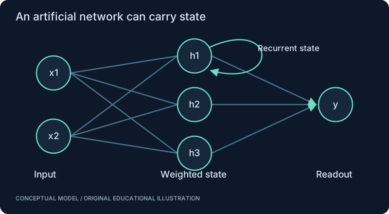
Each robot might use a small controller with its own internal state while sharing parameters or limited messages. Spikes are one possible local representation; simple rules may work equally well. The example uses an ideal synchronous consensus update with access to a shared mean. It illustrates convergence, not a fully decentralized swarm implementation.
SEE THE RELATIONSHIPS
From structure to behavior.
MAKE THE IDEA PRECISE
The mathematics.
| Symbol | Meaning |
|---|---|
| x_i | Scalar state of agent i |
| alpha | Mixing factor between zero and one |
| mean(x) | Mean of the states available to this illustrative update |
Build the equation, step by step
- Compute the mean of the current states and update all agents from that same snapshot. In-place sequential updates would define a different process.
- The formula moves each value a fraction α toward the mean. With 0 < α < 1, each new value lies between its old value and the current mean.
- For this all-to-all toy rule, the mean is preserved and deviations from it shrink by 1 − α. A genuinely local network requires a neighborhood graph and appropriate connectivity/weight conditions.
WORK THROUGH THE NUMBERS
Worked example
States [0, 1, 2] have mean 1. With alpha = 0.5, the next states are [0.5, 1, 1.5]. Disagreement decreases while the mean remains 1 in this ideal case.
A small Python experiment.
Python 3 · Standard library only · Synthetic educational example. Run this in your own notebook or a local file.
states, alpha = [0.0, 1.0, 2.0], 0.5
mean = sum(states)/len(states)
updated = [(1-alpha)*x + alpha*mean for x in states]
print(updated)
Expected output
[0.5, 1.0, 1.5]
Change one quantity, predict the result, and then run the code again. Explain any difference before adding complexity.
Test your understanding.
Try it: Give one agent a stale mean. Does the mean-preservation argument still hold?
Self-check: Is computing a global mean a decentralized algorithm?
Not by itself. Every agent needs access to that mean through some communication mechanism. The example explains consensus arithmetic; a distributed implementation must specify what each agent can observe, how messages travel and what happens when links fail.
Where this model stops: Global averaging is an idealization; real local communication requires graph and delay analysis.
A research question: Does a neural local controller outperform simple rules under matched bandwidth and noise?
Record evidence in your mastery worksheet →THE NEXT LAYER
Chapter depth map.
This introduction provides a first model. The following chapters are outlines for deeper future editions; their full treatments have not yet been published.
Local interactions
19.1 Rules and emergence · Outline
- 19.1.1 Swarm robotics and multi-agent systems
- 19.1.2 Alignment, cohesion and separation
- 19.1.3 Stigmergy and environmental traces
- 19.1.4 Distributed decision-making
- 19.1.5 Emergent patterns need quantitative descriptions
19.2 Communication and decentralization · Outline
- 19.2.1 Local neighborhoods and message budgets
- 19.2.2 Consensus and delays
- 19.2.3 Partial information and conflicting objectives
- 19.2.4 Faults, packet loss and unreliable peers
- 19.2.5 Compare centralized and decentralized control
Neural swarms as experiments
19.3 A small SNN per robot · Outline
- 19.3.1 Observation encoding and local policy
- 19.3.2 Shared parameters versus independent state
- 19.3.3 Local communication as input
- 19.3.4 Group objectives and credit assignment
- 19.3.5 Separate biological analogy from engineered coordination
19.4 Evaluate collective behavior · Outline
- 19.4.1 Coverage, task completion and collision metrics
- 19.4.2 Scaling agent count and bandwidth
- 19.4.3 Randomized starting conditions
- 19.4.4 Robustness to failed robots
- 19.4.5 Baselines with simple local rules
Read with the original sources.
These readings support the concepts and deeper investigation. The worked numbers and illustrations above are teaching examples.
Primary paper / preprint
Schulman et al. (2017): Proximal Policy Optimization Algorithms ↗
Read after policy gradients. Explain the clipped objective and assess results under matched environment and training budgets.